7 Graphing Functions

Graphs are fundamental tools for inspecting and communicating with data.

We begin by importing the pyplot plotting library along with numpy.

import matplotlib.pyplot as plt
import numpy as np

7.1 Graphing Functions

To graph a function, we need a set of \(x\) input values with corresponding \(y\) output values. We can generate a linearly spaced sequence with the np.linspace function. Here is how we might graph \(\sin(x)\) from \(x=0\) to \(x=10\):

# Data
x = np.linspace(0, 10, 100)
y = np.sin(x)

# Create and display the plot
plt.plot(x, y)
plt.show()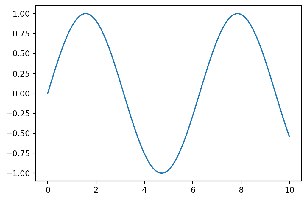

We can turn on plt.grid(), or if we just want \(x\) and \(y\) axes, use:

# Data
x = np.linspace(0, 10, 100)
y = np.sin(x)

# Create and display the plot
plt.axhline(0)
plt.axvline(0)
plt.plot(x, y)
plt.show()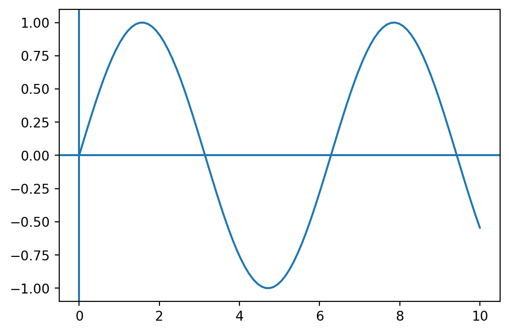

Something interesting happens when we use fewer \(x\) values. Here is the same function with only 8 points:

# Data
x = np.linspace(0, 10, 8)
y = np.sin(x)

# Create and display the plot
plt.plot(x, y)
plt.show()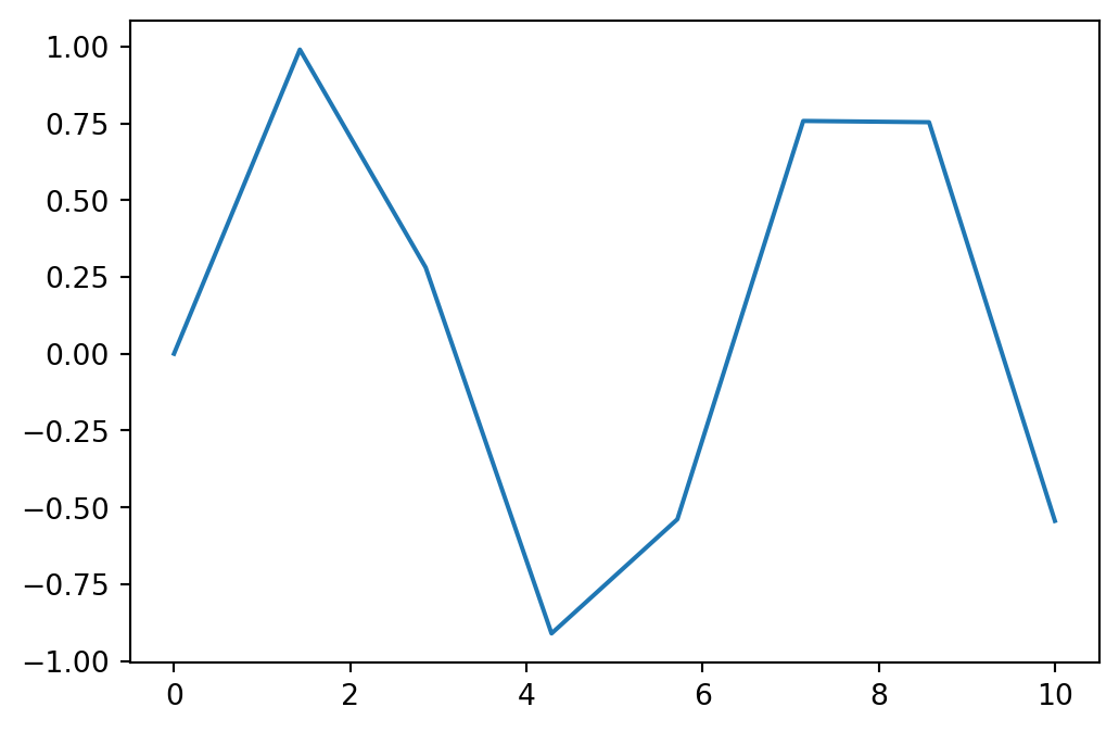

The plt.plot function plots the points given and then connecting those points by lines. That means the points are accurate representations of the function but the lines between the points are approximations.

7.2 Tangent

Tangent is a particularly instructive example. When we graph \(\tan(x)\) it might look like this:

x = np.linspace(-2*np.pi, 2*np.pi, 500)
y = np.tan(x)

plt.plot(x, y)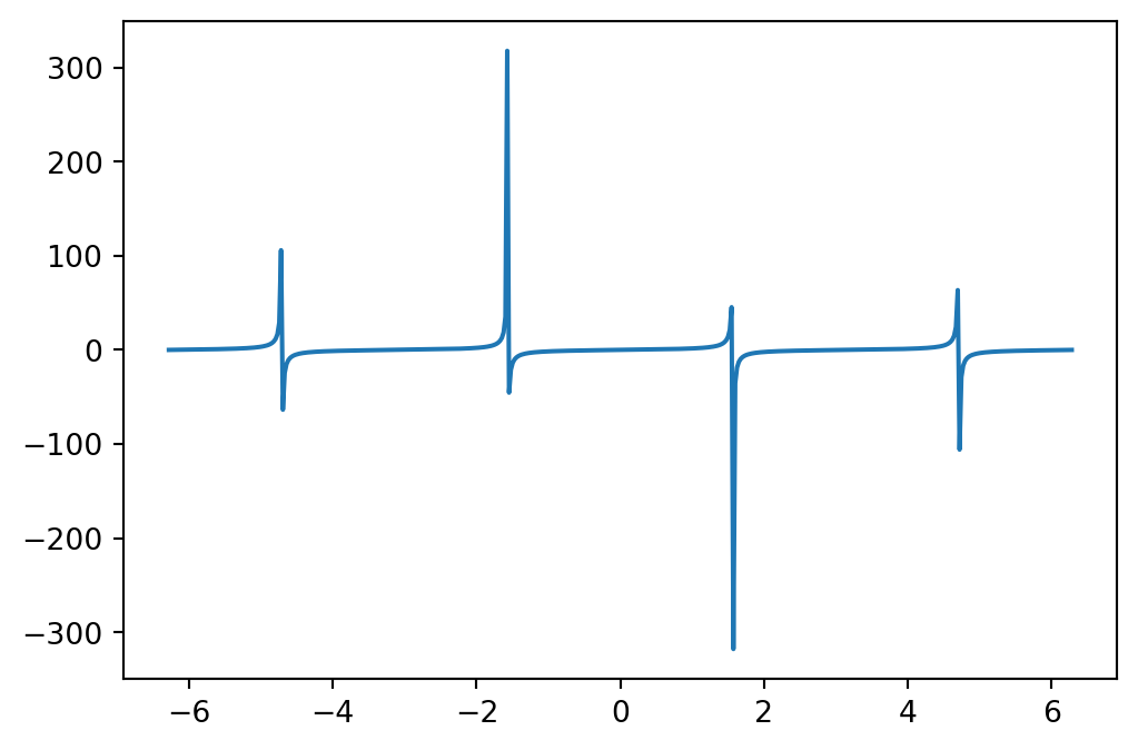

Which leads to some observations:

The infinite discontinuities don’t seem to actually go to infinity here.
Even though they don’t go to infinity, they go far, which stretches the window in the \(y\) direction.
The discontinuities are connected when they shouldn’t be.

For observation 1., we aren’t evaluating \(\tan\) at exactly \(\frac{\pi}{2}\), and we aren’t getting a \(y\) “value” of \(\infty\).

For observation 2. we can adjust our window using np.xlim and np.ylim. Let’s graph \(\tan\) again, but this time constrain the window in the y direction:

x = np.linspace(-2*np.pi, 2*np.pi, 500)
y = np.tan(x)

plt.plot(x, y)
plt.ylim([-10,10])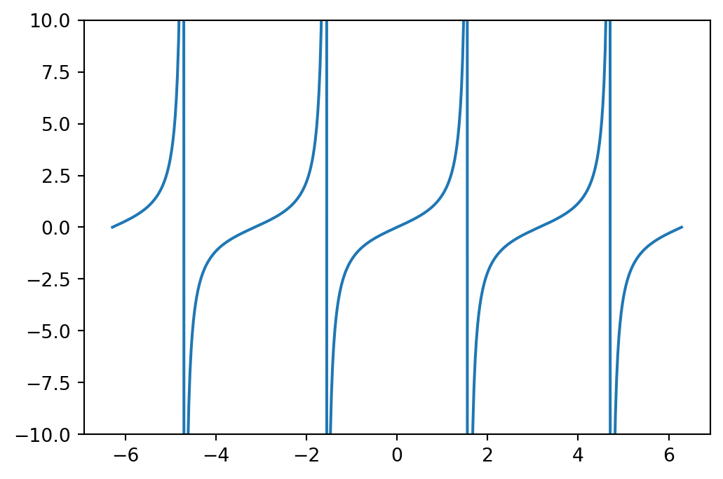

This is nice, but to address observation 3., those infinite discontinuities are still connected. Well, that might be okay if we understand what we are looking at. Alternatively, we could avoid connecting the lines by using a dense scatter plot, a scatter plot with lots of markers:

x = np.linspace(-2*np.pi, 2*np.pi, 10000)
y = np.tan(x)

plt.plot(x, y, '.', markersize=1)
plt.ylim([-10,10])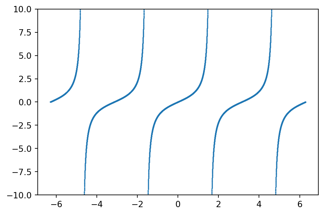

7.3 Examples

Below are several example graphs.

x = np.linspace(-3,3,100)
y = x**2 - 4

plt.grid()
plt.axhline(0, color='black')
plt.axvline(0, color='black')
plt.plot(x,y, linewidth=3)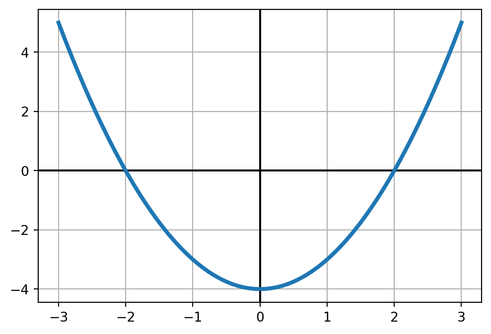

x = np.linspace(0,20,100)
y = x + np.sin(x)

plt.axhline(0, color='black')
plt.axvline(0, color='black')
plt.plot(x,y, color='orange')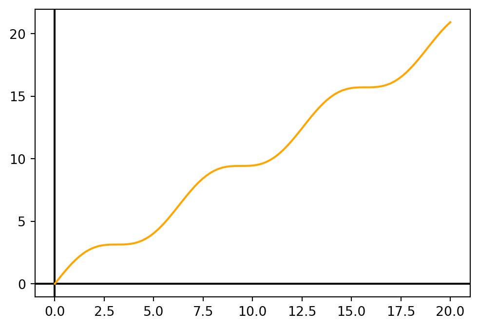

x = np.linspace(0,10,100)
y = np.exp(-x)

plt.axhline(0, color='black')
plt.axvline(0, color='black')
plt.plot(x,y)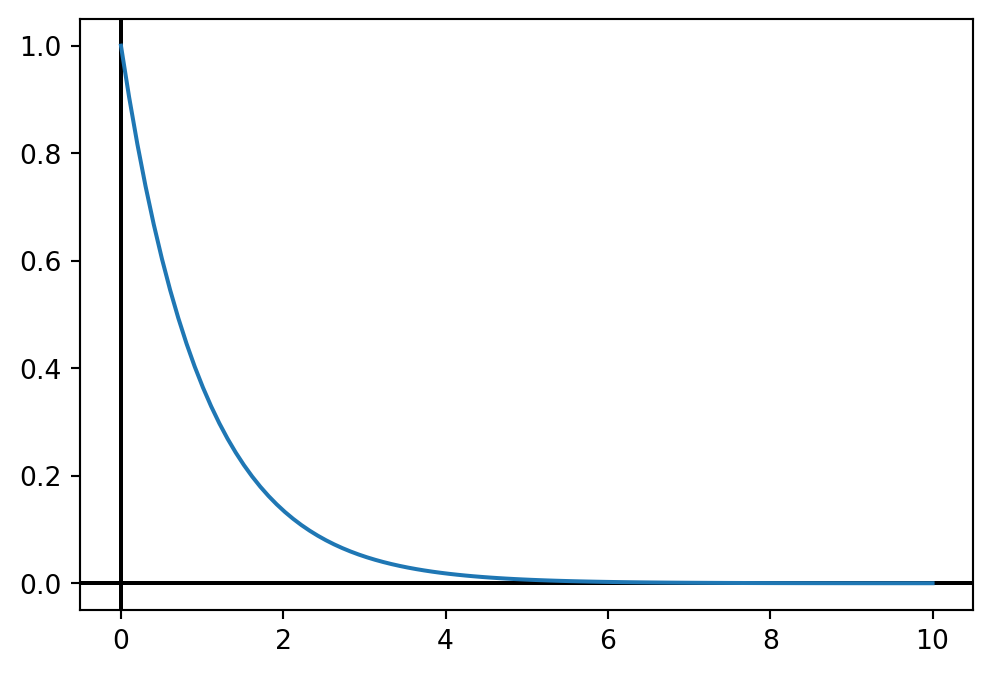

# x and y values 
x = np.linspace(0,2,100)
y1 = np.exp(-x)
y2 = np.sin(x) 
y3 = np.cos(x) 

# Draw the axes 
plt.axhline(0, color='black')
plt.axvline(0, color='black')

# Plot the functions 
plt.plot(x,y1)
plt.plot(x,y2)
plt.plot(x,y3)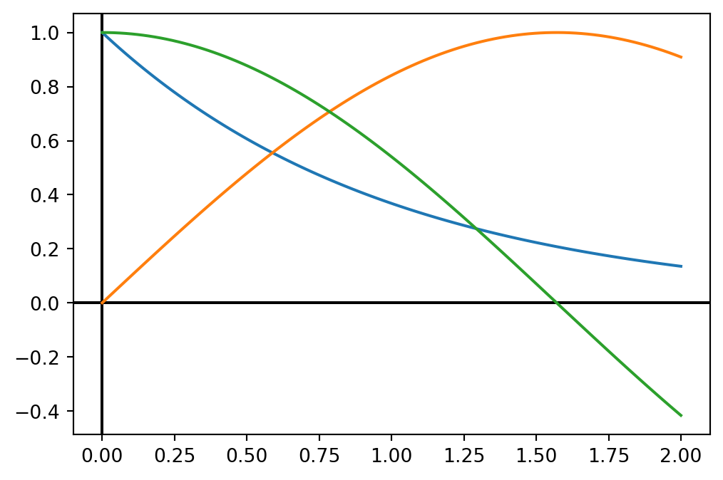

7.4 Graphing Summary

A function graphing template might look something like this:

import numpy as np 
import matplotlib.pyplot as plt 

# x,y data 
x = np.linspace(-10,10, 500)
y = x * np.sin(x)

# Turn on x-y axes 
plt.axhline(0, color='black')
plt.axvline(0, color='black')

# Plot 
plt.plot(x, y)

# Window 
plt.xlim([-10, 10])
plt.ylim([-10, 10])

# Labels 
plt.xlabel('x')
plt.ylabel('y') 
plt.title('x sin(x)')

plt.show()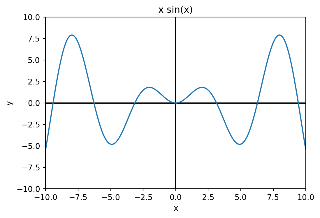

Exercises

Plot each of the following functions over the interval \(-10 \leq x \leq 10\).
1. \(\quad x^3 - 3x\)
2. \(\quad \frac{1}{1+x^2}\)
3. \(\quad x \sin(x)\)
4. \(\quad \frac{1}{x-2}\)
5. \(\quad |x+3|\)
6. \(\quad \cos(x) + x/3\)
Plot \(f(x)=x^2\) on the interval \([-4,4]\). Plot each of the following on the same graph but in a different line style (and / or color), and describe how each differs geometrically from \(f(x)\):
1. \(\quad (x-2)^2\)
2. \(\quad x^2 - 2\)
3. \(\quad x^2 + 3\)
4. \(\quad 2x^2\)
5. \(\quad -x^2\)
The function \(f(x)=\frac{1}{x}\) is undefined at \(x=0\). When we graph this function from \(-1\) to \(1\), we don’t always get an error. For example,
```
x = np.linspace(-1,1,50)
y = 1/x 
```
evaluates with no warning, while
```
x = np.linspace(-1,1,51)
y = 1/x 
```
will give the warning:
```
<python-input-10>:1: RuntimeWarning: divide by zero encountered in divide
```
Explain why undefined functions might sometimes run into warnings and sometimes not.
Graph the functions \(\sin\), \(\cos\), and \(\tan\) on the same plot. Be sure that your plot has reasonable bounds so the functions can be clearly viewed (don’t let the vertical asymptotes of \(\tan\) dominate the vertical zoom).
Under-sampling can dramatically distort our perception of a function. Plot \(f(x)=\sin(2\pi x)\) on \([0, 10]\) using:
1. 11 points
2. 20 points
3. 1000 points
Describe each plot and why it is important to use enough samples when inspecting a function.
The function \[f(x)=\sin\left(\frac{1}{x}\right)\] has some interesting behavior around \(x=0\). Create graphs of \(f(x)\) on the interval \([-1,1]\) using 10, 100, 1000, 10000 points. How many points is enough?
The solution to \[\cos(x) = x\] cannot be found algebraically. However, we can search for an approximate solution by inspecting the graph where \(y=\cos(x)\) intersects \(y=x\). Plot these two functions and use plt.xlim and plt.ylim to “zoom” on any points of intersection to estimate their \((x,y)\) coordinate.